Results

Who influences the market?

In order to identify those people who might influence the stock market, we decided to make two different analyses. The first one consists on finding the speakers whose sentiment expressed in their quotes correlates significantly with the daily variation of the stock market value. In the second analysis, instead, we look for those speakers for which it holds that when they publish sentiment-carrying words the stock market experiences a larger-than-average volume of traded shares. We then study for each speaker the correlation between the number of non-neutral quotes and the volume of shares traded, i.e. positive and negative quotes are treated equally.

1. The idea of the first analysis is to detect if a speaker’s sentiment could impact negatively or positively the value of the market. We firstly transform the positive, negative and neutral values of the sentiment analysis into integers: 1,-1 and 0, respectively. Since many speakers have multiple quotes per day, we decided to set as daily sentiment the sum of the sentiments of all the quotes published in the same date because we believe that if a sentiment is repeated it should impact more on the daily market variation. At this point, we evaluated the Spearman rank correlation between the sentiment vector and the daily stock variation vector. We used the Spearman rank correlation to detect also non-linear correlations. We apply this procedure for all the speakers.
2. The idea of the second analysis is to detect if, for each speaker, the number of sentiment-carrying quotes published has an impact on the volume of shares traded. Here we don’t make a difference between positive and negative quotes because both, if influential, will lead to an increase in the volume traded. So, for this analysis we set as quotes vector the one having as component the sum of all positive and negative daily quotes. We perform a one sided t-test for each speaker (where the alternative hypothesis states that volume values associated with dates with no quotes are statistically smaller) in order to compare the mean value of the volume of the days when some non-neutral quotes have been published with the mean of the other days. Since the mean is not robust to outliers, we remove them based on the interquantile range.

We now compare the results obtained with these two methods. Ideally, we would like to select those individuals who display both a correlation significantly different than zero and a small p-value for the t-test in the second analysis. The scatter graph below represents what we obtained, the x-axis represents the p-value of the t-test of point 2, while the y-axis represents the p-value of the Spearman rank test of point 1. The colors encode the Spearman correlation coefficients of the first analysis.

As we can see, there are no people that have a low p-value in both tests (so placed in the bottom-left corner), but for instance there are people with low p-value in the single tests. Additionally, the two analysis seem not to be correlated, in fact, if we focus on data with the second analysis t-test p-value bigger than 0.95 their first method p-values seem to be uniformly distributed.

How influential are the most influential speakers? And who are they?

After this analysis we decided to focus on the second method because we believe that due to its assumptions it is less likely to be incorrect. For instance, the first analysis is much more dependent on the sentiment analysis which could fail in two ways. First, sentiments detected might be incorrect for some speakers biasing the results. Secondly, we only associated to quotes a positive or negative value, without specyfing how much positive or negative they are which could lead to less precise results. Consequently, from now onwards we will continue the analysis only with the speakers that display a pvalue of the t-test in the second analysis smaller than 0.1, i.e., those individuals whose quotes seem to cooccur with larger-than-average volumes.

We are left with eight speakers. These eight seleceted people could potentially have an impact on the S&P500. In order to study how impactful these individuals are we compute the Spearman rank correlation between the number of non-neutral daily quotes and the daily stock market volume. From the results only one of them has a a negative correlation, meaning that he doesn’t have an impact on it. While the other seven people have positive coefficients and a significant p-value, so we believe that these speakers could have had an impact on the stock market volume. We now present some of them.

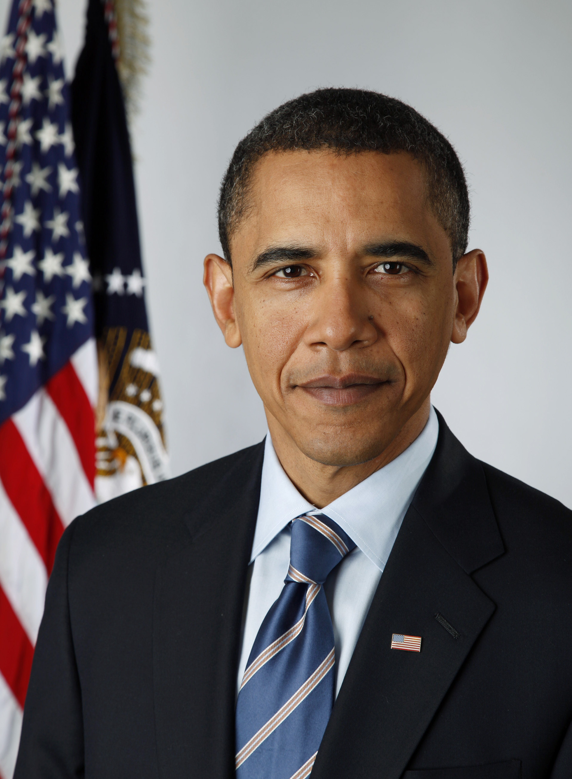
• Barack Obama

Barack Obama is a politician, in particular he was president of the United States of America from 2009 to 2017. So it’s reasonable to think that he could have an impact on the market. In the timeseries below we show the graphical correlation between the amount of quotes and the stock volume. What is interesting to notice is that the amount of quotes is higher in the first two years (so his last years of charge).

• Hillary Clinton

Hillary Clinton is a politician, she has had an important role in the american gouvernment. As we can notice in the timeseries below, she has the highest amount of quotes between mid 2015 and 2017, so during the election campaign with the democratics against Trump.

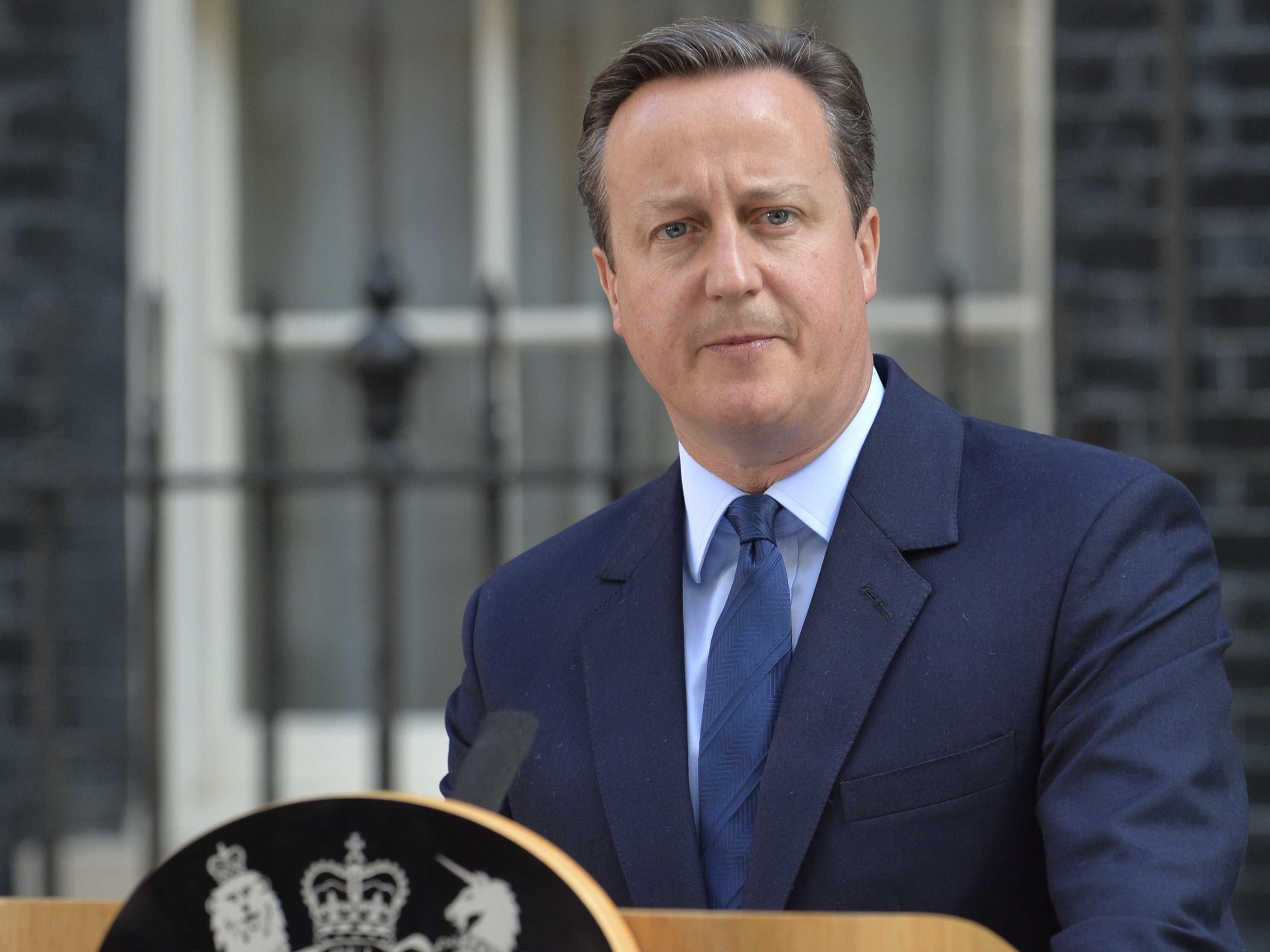
• David Cameron

David Cameron is a politician, he was the Britain prime minister from 2010 to 2016. We again noticed that he was more active during the years of his charge.

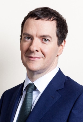
• George Osborne

Geroge Osborne is a politician, he’s a member of the Britain conservative party, in particular he was Chancellor of the Exchequer from 2010 to 2016, meaning that he was the finance minister of England during those years. In fact, as it is shown in the graphic below, he has his highest peaks during those years.